Decision Trees

Jan 31, 2018 12 min read Deep Learning

Have you been struggling to learn about what decision trees are? Finding it difficult to link pictures of trees with machine learning algorithms? If you answered yes to these questions then this post is for you.

Decision trees are an amazingly powerful predictive machine learning method that all Data Analysts should know. When I was researching tree-based methods I could never find a hand worked problem. Most other souces simply list the maths, or show the results of a grown tree. To truly understand the method though I needed to see how trees are actually grown! So I worked it out and now to save time for you I have put my working into this post.

The majority of the theory involved in this post is thanks to this paper (Breiman et al. 1984) whilst the mathematics is taken from (Friedman, Hastie, and Tibshirani 2001).

The structure of this post follows closely to how I learn, and how I hope you learn! First I will list examples of how decision trees have been used and their advantages and disadvantages. Next Ill present a worked example and following will be an example of classification and regression example.

Examples

Decision Trees are used in a wide variety of fields! These examples are in credit to Micheal Dorner. I have used decision trees in my Masters thesis too.

Astronomy: Distinguishing between stars and cosmic rays in images collected by the Hubble Space Telescope.
Medicine: Diagnosis of the ovarian cancer.
Economy: Stock trading.
Geography: To predict and correct errors in topographical and geological data.
Personally: Predict the probabilities of winning for teams in professional Dota 2 matches.

Table of advantages and disadvantages

Advantages	Disadvantages
Easy to understand	Overfits the training data
Resistant to outliers and weak features	Stuggles with continuous depedent variables
Easy to implement in practice	Need important variables
Can handle datasets with missing values and errors	Trees are unstable
Makes no assumptions about the underlying distributions	Lack of smoothness

Advantages:

Easy to understand: When a decision tree is constructed you can view the decision rules in a nice looking tree diagram, hence the name!
Resistant to outliers and weak features: The splitting criteria does not care greatly how far values are from the decision boundary. The splitting criteria splits according the strongest features first which minimises the harm of the weak features (the weak features are splitting already split data = smaller effect).
Easy to implement in practice: As the model is resistant to outliers and weak features in practice you do not need to spend as much time testing different feature input combinations.
Can handle datasets with missing values and errors: Similar to being resistant to outliers and weak features.
Makes no assumptions about the underlying distributions: This may not so important in practice but it makes the model theorectically more appealing.

Disadvantages:

Overfits the training data: This is a very large issue but can be minimised using random forests. Which we will cover in the next post.
Stuggles with continuous depedent variables: Due to the leafs containing several observations which are averaged the prediction space is not smooth. This makes highly accurate regression predictions difficult to achieve.
Need important variables: Without strong predictors tree based methods lose many of their strengths.
Trees are unstable: The structure of an estimated tree can vary significantly between different estimations.

The Algorithm

Start at the root node.
For each input, find the set \(S\) that minimizes the sum of the node impurities in the two child nodes and choose the split \(\{X \in S \}\) that gives the minimum overall \(X\) and \(S\).
If a stopping criterion is reached, exit. Otherwise, apply step 2 to each child node in turn.

In simplier words to build the tree you need to decide where the splits(branches) are going to happen. You need to calculate for each possible split for each input variable an ‘impurity’ measure. For classification trees this impurity measure can be the Gini Index. This is just a measure that says how well the split divides the data. The smallest impurity score is where the split will happen.

After you have divided the data into two regions you continue to split those regions again and again until you reach some stopping rule. Once the stopping rule is reached it is possible to prune the tree. This is typically done occuring to some cost complexity measure where non-terminal splits can be removed.

Splitting criteria - Gini Impurity

There are several splitting criteria that can be used but I will be using the Gini method for this worked example. We can define the Gini Impuirty as:

\[ GiniImpurity = \sum_{k \neq k'} \hat{p}_{mk}\hat{p}_{mk'} = \sum^{K}_{k=1} \hat{p}_{mk}(1-\hat{p}_{mk}) \] where

\[ \hat{p}_{mk} = \frac{1}{N_{m}}\sum_{x_{i}\in R_{m}} I(y_{i} = k) \] and

\[ N_{i} = \#\{x_{i} \in R_{m} \} \] and

\[ R_{1}(j,s) = \{X|X \leq s \} \]

\[R_{2}(j,s) = \{X|X > s \} \]

Stopping criteria - Minimum Leaf Size

There are several possible rules for when the splitting algorithm should stop. These possibilities include:

If a split region only has identical values of the dependent variable then that region will not be split any futher.
If all cases in a node have identical values for each predictor, the node will not be split.
If the current tree depth reaches the user-specified maximum tree depth limit value, the tree growing process will stop.
If the size of a node is less than the user-specified minimum node size value, the node will not be split.
If the split of a node results in a child node whose node size is less than the user-specified minimum child node size value, the node will not be split.

Other stopping criteria could include an error minimisation rule, but this tends to miss important splits that could happen. That is why it is preferable to grow the tree and then prune it back to an acceptable level. For this tutorial a minimum leaf size of 5 was chosen.

Prunning Criteria - Misclarification Rate

\[ \frac{1}{N_{m}} \sum_{i \in R_{m}} I(y_{i} \neq k(m)) = 1 - \hat{p}_{mk(m)} \] where

\[ k(m) = argmax_{k}\hat{p}_{mk} \]

Worked Example

Let us begin with a worked simple example. It always helps to understand the intuition to see the basics of the method being used.

Lets us build a simple dataset to work the problem by hand. The dataset will be ten observations of two classes, 0 or 1, with two predictors, X1 and X2.

Class <- as.factor(c(0,0,0,0,0,1,1,1,1,1)) # The 2 class vector
X1 <- c(4,4.5,5,5.5,3,5.6,6,6.5,6.2,5.9) # Random values for predictor 1
X2<- c(9,10,11,10,9,8,7,8,7,8) # Similarly
df <- cbind.data.frame(Class, X1, X2) # Combine the class vector and the two predictors

ggplot(data = df, aes(x = X1, y=X2)) + # Plot the two predictors and colour the 
  ggtitle(label = "The two Predictors with their assoicated Class values") +
  geom_point(aes(color=Class), size = 6, alpha = .5) # observations according to which class they belong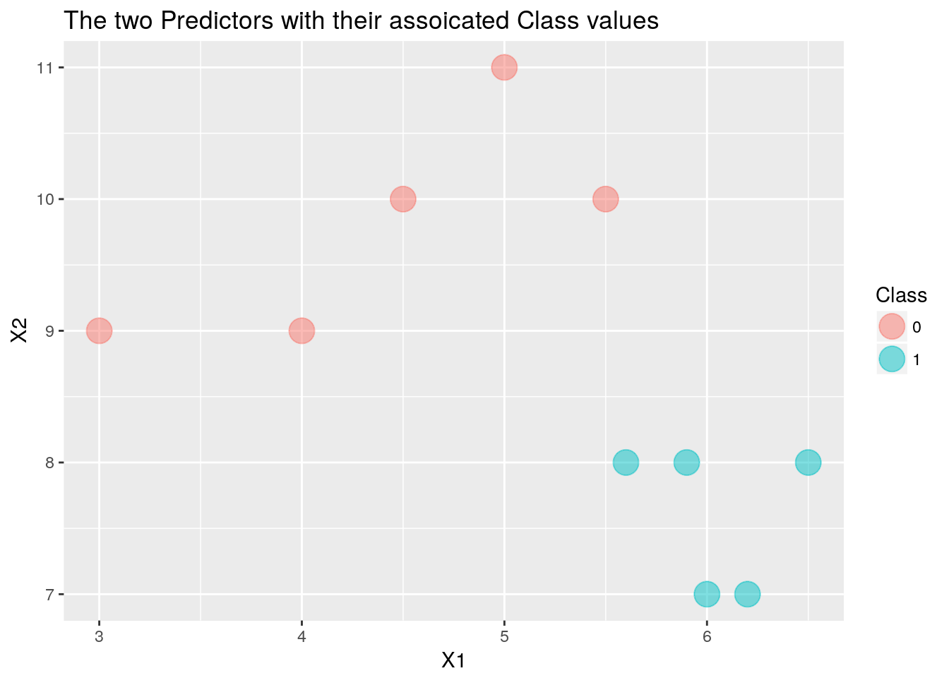

From the graph it is obvious how to split the data but lets us worked it out using the algorithm to see how it works. First we will calculate the Gini Impurity for each possible split in the range of each predictor.

Predictor1test <- seq(from = 3, to = 7, by  = 0.1) # The potential splits where we calculate the Gini Impurity
Predictor2test <- seq(from =7, to = 11, by = 0.1) # Similar for Predictor 2
CalculateP <- function(i, index, m, k) { # Function to calculate the proportion of observations in the split
  if(m=="L") {                          # region (m) which match to class (k) 
    Nm <- length(df$Class[which(df[,index] <= i)]) # The number of observations in the split region Rm
    Count <- df$Class[which(df[,index] <= i)] == k # The number of observations that match the class k
  } else {
    Nm <- length(df$Class[which(df[,index] > i)])
    Count <- df$Class[which(df[,index] > i)] == k
  } 
  P <- length(Count[Count==TRUE]) / Nm # Proportion calculation
  return(c(P,Nm)) # Returns both the porportion and the number of observations
}
CalculateGini <- function(x, index) { # Function to calculate the Gini Impurity
  Gini <- NULL # Create the Gini variables
  for(i in x) {
    pl0 <- CalculateP(i, index, "L", 0) # Proportion in the left region with class 0
    pl1 <- CalculateP(i, index, "L", 1)
    GiniL <- pl0[1]*(1-pl0[1]) + pl1[1]*(1-pl1[1]) # The Fini for the left region
    pr0 <- CalculateP(i, index, "R", 0)
    pr1 <- CalculateP(i, index, "R", 1)
    GiniR <- pr0[1]*(1-pr0[1]) + pr1[1]*(1-pr1[1])
    Gini <- rbind(Gini, sum(GiniL * pl0[2]/(pl0[2] + pr0[2]),GiniR * pr0[2]/(pl0[2] + pr0[2]), na.rm = TRUE)) # Need to weight both left and right Gini scores when combining both
  }
  return(Gini)
}
Gini <- CalculateGini(Predictor1test, 2)
Predictor1test<- cbind.data.frame(Predictor1test, Gini)
Gini <- CalculateGini(Predictor2test, 3)
Predictor2test<- cbind.data.frame(Predictor2test, Gini)

ggplot(data = Predictor1test, aes(x=Predictor1test, y=Gini)) + 
  ggtitle("Gini Index For Possible Values Of X1") +
  geom_line()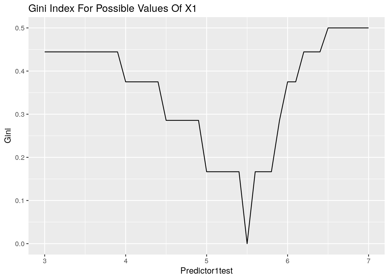

We can see that the most pure split for predictor1 is at 5.5. All other splits leave some impurity in the resulting spaces.

ggplot(data = Predictor2test, aes(x=Predictor2test, y=Gini)) + 
  ggtitle("Gini Index For Possible Values Of X2") +
  geom_line()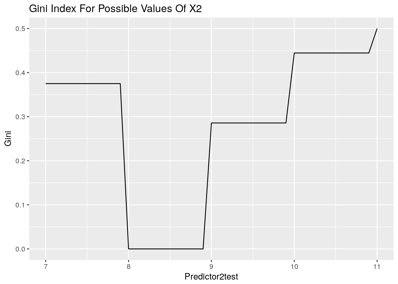

Here we can see a region where the Gini Impurity is minimised. Any value here would be suitable. Now we can observe a hand calculation of the Gini Impurity for X1 = 5.5.

With a minimum off 5 observations per leaf we are already at the stopping criteria but let us see the misclassification for each off our potential stopping criteria for the sake of illumination. Also due to the purity of the split we do not need to prune the tree.

CalculatePkm <- function(i, index, m) { # This is different to the other P function is that it calculates the proportion to
  if(m=="L") {                          # only the majority class
    Nm <- length(df$Class[which(df[,index] <= i)]) 
    Km <- as.integer(names(sort(table(df$Class[which(df[,index] <= i)]), decreasing = TRUE)[1]))
    Count <- df$Class[which(df[,index] <= i)] == Km
  } else {
    Nm <- length(df$Class[which(df[,index] > i)])
    Km <- as.integer(names(sort(table(df$Class[which(df[,index] > i)]), decreasing = TRUE)[1]))
    Count <- df$Class[which(df[,index] > i)] == Km
  } 
  P <- length(Count[Count==TRUE]) / Nm
  return(c(P,Nm))
}
CalculateMissClass <- function(x, index) {
  miserr <- NULL
  for(i in x) {
    pLkm <- CalculatePkm(i, index, "L")
    missclassL <- (1 - pLkm[1])
    pRkm <- CalculatePkm(i, index, "R")
    missclassR <- (1 - pRkm[1])
    miserr <- rbind(miserr,  sum(missclassL * pLkm[2]/(pLkm[2] + pRkm[2]),missclassR * pRkm[2]/(pLkm[2] + pRkm[2]), na.rm = TRUE))
  }
  return(miserr)
}
miserr <- CalculateMissClass(Predictor1test[,1], 2)
Predictor1test<- cbind.data.frame(Predictor1test, miserr)
miserr <- CalculateMissClass(Predictor2test[,1], 3)
Predictor2test<- cbind.data.frame(Predictor2test, miserr)

ggplot(data = Predictor1test, aes(x=Predictor1test, y=miserr)) + 
  ggtitle("Misclassification Error for X1") +
  geom_line()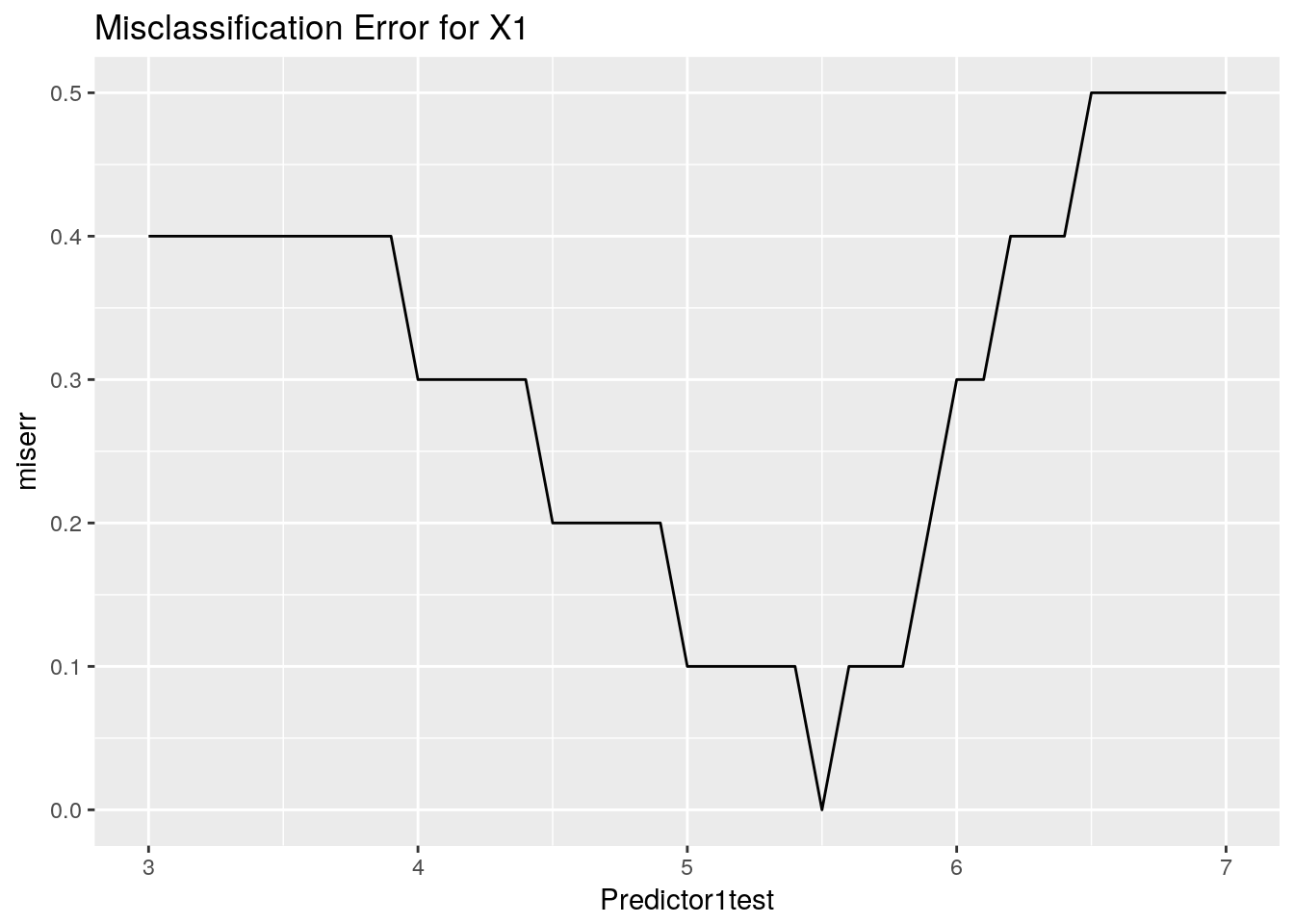

ggplot(data = Predictor2test, aes(x=Predictor2test, y=miserr)) + 
  ggtitle("Misclassification Error for X2") +
  geom_line()

Similar to the case with the Gini Impurity we can see the regions where the measure is minimised. Now we can go through a hand drawn problem and see the calculation in action.

Now with such a small dataset it does not make sense to prune the tree but let us continue to see an example with real data.

Example: Classification Tree

For this example we will use the iris dataset that comes packed with R. There are three species of the iris flower: setosa, versicolor, and virgincia. We will use the classification tree process to separate the feaures of Sepal Length, Sepal Width, Pdeal Length, and Petal Width.

Species of Iris with each Predictor Combination

Iris data plotted with each combination of predictor

From the data you can see that Setosa can be separated easily from the other two species. Try it yourself, where would you draw the line to separate Setosa?

Build the tree

Now that we have worked through how the classification tree is grown we can resort to using already established packages to estimate our decision tree for us. I will be using the rpart package for this post but there are many other packages that can estimate trees.

Tree <- rpart(Species ~ ., data=iris, parms = list(split = 'gini') )

The Splits

The tree growing process can involve many more splits than the single split from our hand worked problem. Here we can see all the splits that were done when growing this tree.

kable(Tree$splits, digits = 2, format = 'markdown')

	count	ncat	improve	index	adj
Petal.Length	150	-1	50.00	2.45	0.00
Petal.Width	150	-1	50.00	0.80	0.00
Sepal.Length	150	-1	34.16	5.45	0.00
Sepal.Width	150	1	19.04	3.35	0.00
Petal.Width	0	-1	1.00	0.80	1.00
Sepal.Length	0	-1	0.92	5.45	0.76
Sepal.Width	0	1	0.83	3.35	0.50
Petal.Width	100	-1	38.97	1.75	0.00
Petal.Length	100	-1	37.35	4.75	0.00
Sepal.Length	100	-1	10.69	6.15	0.00
Sepal.Width	100	-1	3.56	2.45	0.00
Petal.Length	0	-1	0.91	4.75	0.80
Sepal.Length	0	-1	0.73	6.15	0.41
Sepal.Width	0	-1	0.67	2.95	0.28

There are quite a few splits here! So let us look at the two most important splits, Petal.Length = 2.5 and Petal.Width = 0.8.

Where the split happens with PetalLength = 2.5

Where the splits occure when PetalWidth = 0.8

The Final Pruned Tree

rpart.plot(Tree)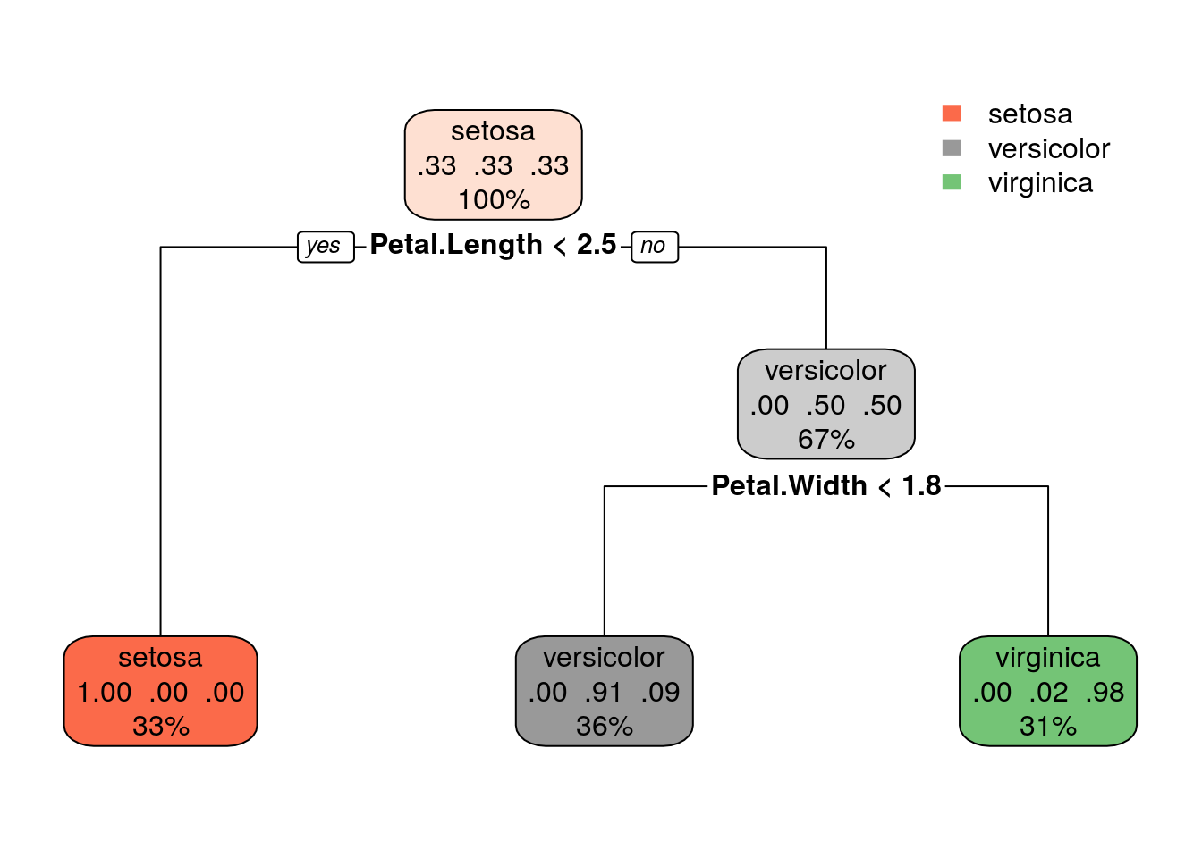

This is the final tree diagram. You may notice that the tree has been pruned to have only 2 split nodes. Indeed can see that the split for Petal.Width is moved to 1.8 instead of at 0.8 in the final decision tree.

Example: Regression Tree

For this example I will be providing less explanation.

Splitting Criteria - Minimising The Sum Of Squares

\[ \min_{j,s} [\min_{c1} \sum_{x_{i} \in R_{1}(j,s)}(y_{i} -c_{1})^2 + \min_{c2} \sum_{x_{i} \in R_{2}(j,s)}(y_{i} -c_{2})^2 ] \]

where

\[ \hat{c}_{m} = \frac{1}{N_{m}} \sum_{x_{i} \in R_{m}} y_{i} \] The equation calculates, for each variable, the sum of squared errors. The value for \(c_{m}\) is simply the average observation value in that region. The algoirthm then finds the smallest sum of squares for that variable and does that for each variable. The algorithm finally compares the champion split from each variable to determine the winner for the overall split to occur. The stopping criteria will once again be a minimum size of terminal nodes to be 5.

Pruning Criteria - Cost Complexity Criteria

Let:

\[ Q_{m}(T) = \frac{1}{N_{m}} \sum_{x_{i} \in R_{m}} (y_{i} - \hat{c}_{m})^2 \]

we may then define cost complexity criterion as:

\[ C_{\alpha}(T) = \sum^{|T|}_{m=1} N_{m}Q_{m}(T) + \alpha|T| \]

Our goal is to minimise this function. The compromise between tree size and its fit to the data is dictated by \(\alpha\). Smaller values lead to larger trees and larger values lead to more pruning.

There are processes by which to estimate \(\alpha\) but we will not go into that today.

The Data: USA Arrests

ggplot(data = USArrests, aes(x = Assault, y = UrbanPop)) + 
  geom_point(aes(color=Murder), size = 6, alpha = .5)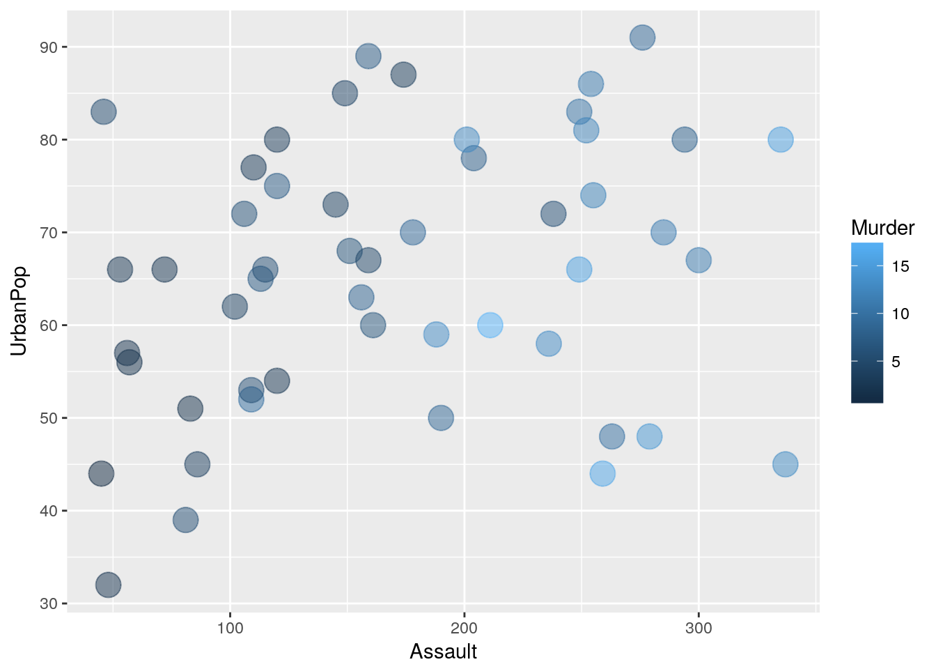

RegressionTree <- rpart(Murder~ Assault + UrbanPop, data=USArrests)
kable(RegressionTree$splits, digits = 2, format = 'markdown')

	count	ncat	improve	index	adj
Assault	50	-1	0.66	176.0	0.00
UrbanPop	50	-1	0.03	57.5	0.00
UrbanPop	0	-1	0.62	69.0	0.14
Assault	28	-1	0.35	104.0	0.00
UrbanPop	28	-1	0.11	58.5	0.00
UrbanPop	0	-1	0.79	51.5	0.45
UrbanPop	22	1	0.26	66.5	0.00
Assault	22	-1	0.04	243.5	0.00
Assault	0	1	0.64	195.5	0.11

The First 4 Splits

The Constructed Tree

rpart.plot(RegressionTree)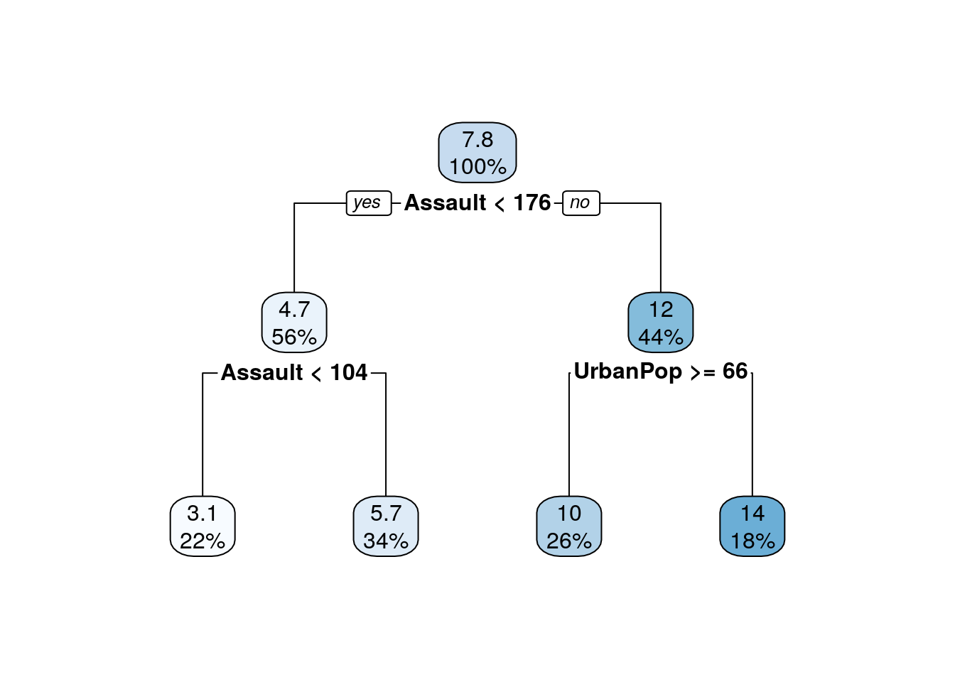

Summary

Next up will be a post on Random Forests. How trees are implemented in the real world.

References

Breiman, Leo, Jerome Friedman, Charles J Stone, and Richard A Olshen. 1984. Classification and Regression Trees. CRC press.

Friedman, Jerome, Trevor Hastie, and Robert Tibshirani. 2001. The Elements of Statistical Learning. Vol. 1. Springer series in statistics New York.

Decision Trees Machine Learning Data Analysis