Introduction
This is going to be part of series where I illustrate examples and questions from the brilliant book by Sutton and Barto Sutton and Barto (1998). You can download the pdf version of the newly updated book online, just google it. I am planning on going through each chapter and illustrating 1 or 2 examples from each chapter.
MultiArmed Bandits
What on earth is a mutliarmed bandit? It might be easier to think of it as which pokie you choose to play on down at the local. Say there are 10 pokies at the pub, then you need to decide which machine to game at. But you don’t know which machine will pay at the most so you need to explore and discover where the odds are at.
Lets as describe a metric; return per dollar spent. That is for every dollar you put in a machine how much do get as a return? (0, 1.5,-.5)
Let us setup 10 pokie machines with normal distributions but with differing mean returns.
rewardMeans <- rnorm(10)
plot(rewardMeans)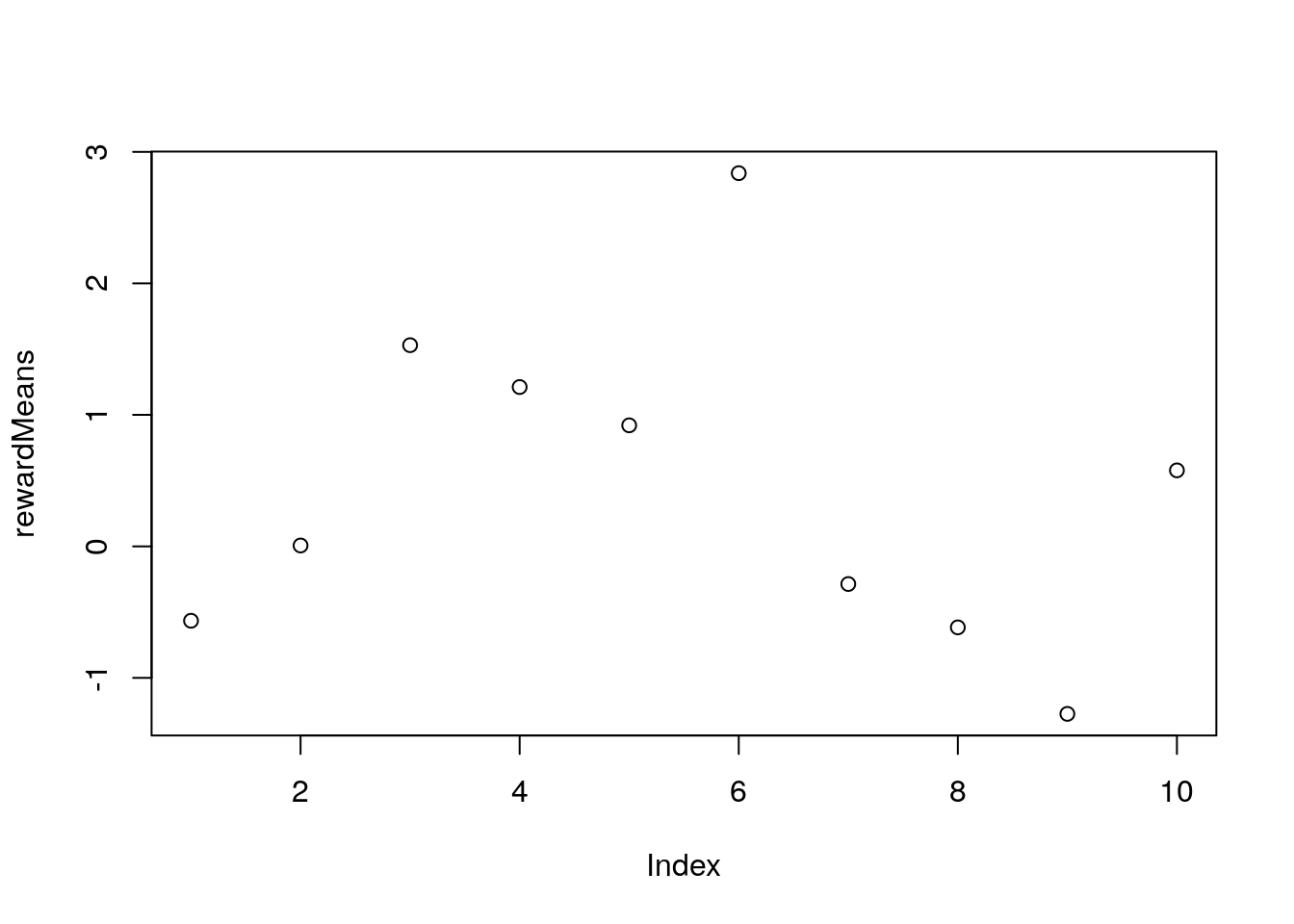
From our little plot we can see that the best pokie is machine 3.
Now let us set up our learning problem for our little agent to learn the best machine.
The algorithm
\[\begin{equation} \text{for the number of actions k, create:} \\ \\ valueFunction(action) = 0 \\ countFunction(action) = 0 \\ \\ Repeat until iteration count is reached: \\\ action <- \begin{cases} \text{The action that maxes the valueFuntion with prob (1 - epsilon)} \\ \text{A random action with prob epsilon} \\ \end{cases}\\ \\ reward <- bandit(action) \\ countFunction(action) += 1 \\ valueFunction(action) += \frac{1}{countFunction(action)}*(reward - valueFunction(action)) \\ \end{equation}\]Programming Example
averagerewardAverage <- vector()
averageactions <- vector()


for(w in 1:500) {
# Setup our functions
# Number of pokies
k <- 10
valueFunction <- vector()
countFunction <- vector()

for(i in 1:k) {
  valueFunction[i] <- 0
  countFunction[i] <- 0
}

# Number of steps
T <- 1000
rewardTotal <- vector()
rewardAverage <- vector()
actions <- vector()
for(x in 1:T) {
  epsilon <- 0.1
  if(epsilon > sample(c(0:9), size=1)) {
    action <- sample(c(1:k), size=1)
  } else {
     action <- which(valueFunction==max(valueFunction))[1]
  }
  actions[x] <- action
  # reward <- bandit(action)
  reward <- rnorm(1, mean=rewardMeans[action])
  rewardTotal[x] <- reward
  rewardAverage[x] <- mean(rewardTotal)
  countFunction[action] <- countFunction[action] +  1
  valueFunction[action] <- valueFunction[action] + (1 / countFunction[action])*(reward - valueFunction[action])
}

averagerewardAverage <- rbind(averagerewardAverage,rewardAverage)
averageactions <- rbind(averageactions, actions)
}

averagerewardAverage <- colMeans(averagerewardAverage)
averageactions <- colMeans(averageactions)
Let us plot our results
plot(averagerewardAverage)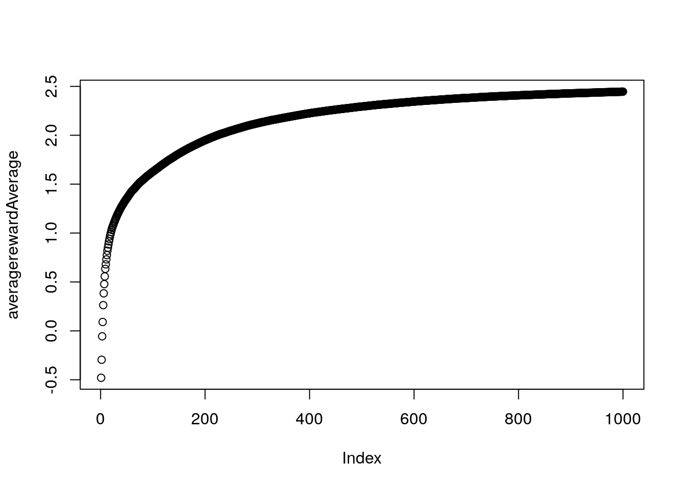
Now considering our best slot machine has a payout of around 1.5 it seems out model is not that great at finding the best machine. This highlights the huge problem with reinforcement learning. That is it is HARD.
Optimistic Initial values with greedy epsilon = 0
averagerewardAverage <- vector()
averageactions <- vector()


for(w in 1:500) {
# Setup our functions
# Number of pokies
k <- 10
valueFunction <- vector()
countFunction <- vector()

for(i in 1:k) {
  valueFunction[i] <- 10
  countFunction[i] <- 10
}

# Number of steps
T <- 1000
rewardTotal <- vector()
rewardAverage <- vector()
actions <- vector()
for(x in 1:T) {
  epsilon <- 0
  if(epsilon > sample(c(0:9), size=1)) {
    action <- sample(c(1:k), size=1)
  } else {
     action <- which(valueFunction==max(valueFunction))[1]
  }
  actions[x] <- action
  # reward <- bandit(action)
  reward <- rnorm(1, mean=rewardMeans[action])
  rewardTotal[x] <- reward
  rewardAverage[x] <- mean(rewardTotal)
  countFunction[action] <- countFunction[action] +  1
  valueFunction[action] <- valueFunction[action] + (1 / countFunction[action])*(reward - valueFunction[action])
}

averagerewardAverage <- rbind(averagerewardAverage,rewardAverage)
averageactions <- rbind(averageactions, actions)
}

averagerewardAverage <- colMeans(averagerewardAverage)
averageactions <- colMeans(averageactions)
Let us plot our results
plot(averagerewardAverage)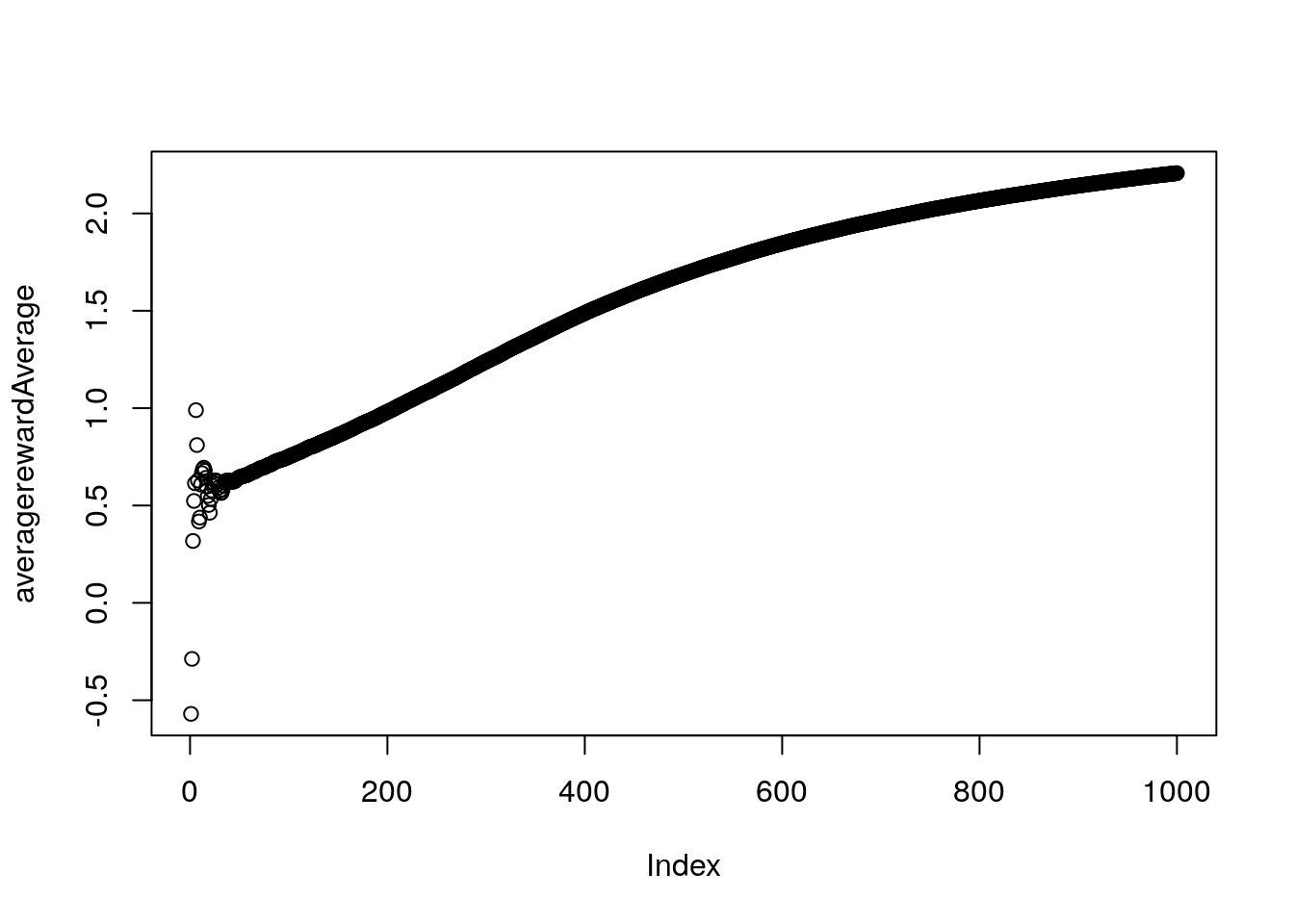
Constant Step Size
averagerewardAverage <- vector()
averageactions <- vector()


for(w in 1:500) {
# Setup our functions
# Number of pokies
k <- 10
valueFunction <- vector()
countFunction <- vector()

for(i in 1:k) {
  valueFunction[i] <- 0
  countFunction[i] <- 0
}

# Number of steps
T <- 1000
rewardTotal <- vector()
rewardAverage <- vector()
actions <- vector()
for(x in 1:T) {
  epsilon <- 1
  if(epsilon > sample(c(0:9), size=1)) {
    action <- sample(c(1:k), size=1)
  } else {
     action <- which(valueFunction==max(valueFunction))[1]
  }
  actions[x] <- action
  # reward <- bandit(action)
  reward <- rnorm(1, mean=rewardMeans[action])
  rewardTotal[x] <- reward
  rewardAverage[x] <- mean(rewardTotal)
  countFunction[action] <- countFunction[action] +  1
  valueFunction[action] <- valueFunction[action] + 0.05*(reward - valueFunction[action])
}

averagerewardAverage <- rbind(averagerewardAverage,rewardAverage)
averageactions <- rbind(averageactions, actions)
}

averagerewardAverage <- colMeans(averagerewardAverage)
averageactions <- colMeans(averageactions)
Let us plot our results
plot(averagerewardAverage)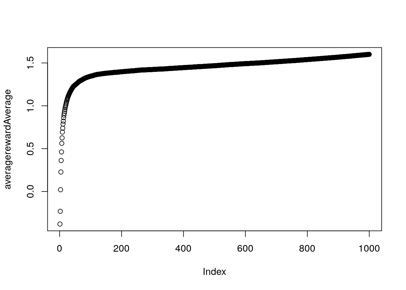
Conclusion
Pretty cool. Next post will be on Markov Decision Processes.
Sutton, Richard S, and Andrew G Barto. 1998. Reinforcement Learning: An Introduction. Vol. 1. 1. MIT press Cambridge.